Why can’t we use Neural Nets?!

One very interesting application of neural network is how we can use it to classify an image. In order to accomplish this, our normal neural network does not suffice because of two reasons.

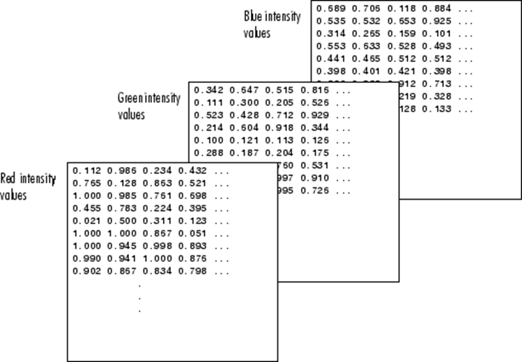
1. Not enough computational power. Computers do not view images like us humans. They see an image as a matrix of numbers where each number corresponds to the pixel value. An image of size 256 x 256 x 3 is a matrix with 3 layers (RGB) where each layer contains 256 x 256 values.

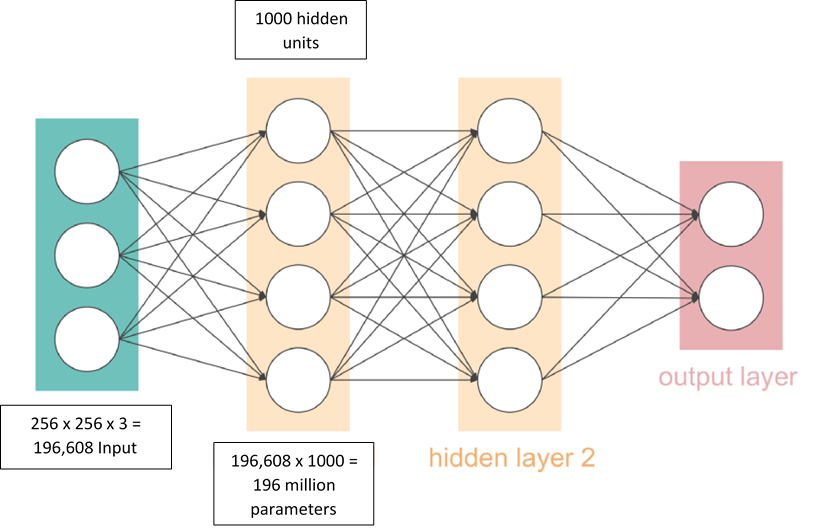
Now, in a normal neural network, we would have to flatten these value into a vector and feed them as input. Let’s do some simple calculations. A color image with size 256 x 256 would have 256 x 256 x 3 input values which is equal to 196,608 inputs. If, for example, we have 1,000 hidden units in our first hidden layer, there would be approximately 196 million parameters or weights for us to train which is infeasible.

2. Local Features Loss. With images, you normally do want to preserve the local features. What we mean by this is if you want to classify a cat, we would like to preserve the key features such as the face or ears of the cat. However, by flattening the matrix, we have removed all those local features which is not a good approach. Even with these obstacles, people have invented a new way to solve these problems with the technique which is known as convolution.

Convolution of Images

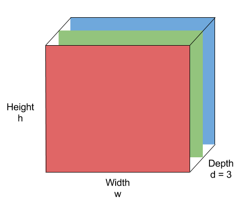
For colored images, the image matrix has a depth of 3, one for each of the three color channels: (R)ed, G(reen), B(lue).

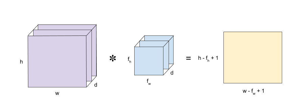
Convolution is a mathematical operation that takes two inputs:

1. An image matrix (volume) of dimension (h x w x d)
2. A filter (fh x fw x d)

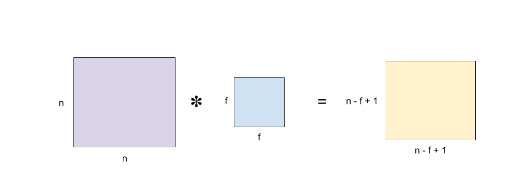
and outputs a volume of dimension (h — fh + 1) x (w — fw + 1) x 1.

In a simplified case where d = 1, h = w = n, and fh = fw = f (meaning that the input image and filter are squared, greyscale images), the output volume dimension simplifies to (n — f + 1) x (n — f + 1).

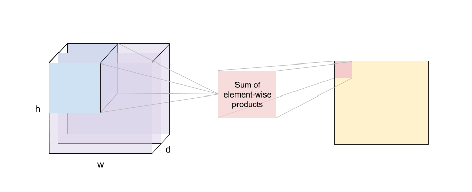
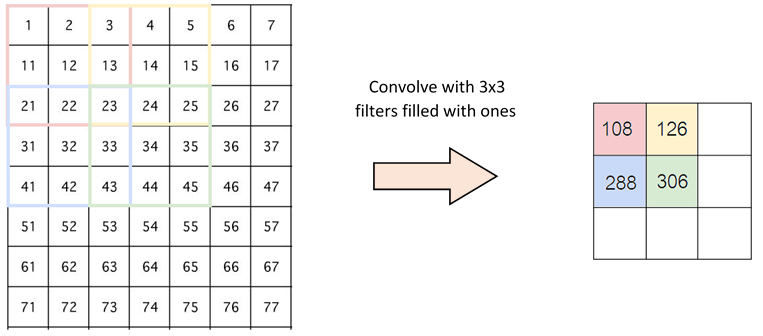
We compute the output of the convolution as follows:

We start with the top-left pixel of the output:

1. “Place” the filter on the top-left corner of the input image
2. Calculate the element-wise product of each corresponding pixel value
3. Sum the products to obtain the top-left pixel value of the output

Next, move the filter to the right by one position and repeat steps 2. and 3. to obtain the next pixel value of the output! Keep doing this until we have fully covered the original input image.

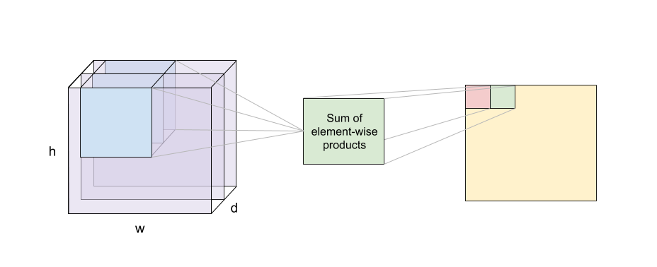
Note that the depth of the input volume and filter must match.

Remark: It is possible that the filter dimension might not fully “fit” the input image. It turns out there are a few ways to overcome this. Padding, discussed in the next section, is one of them.

Remark 2: Actually, the operation we have described above is formally called cross-correlation in the mathematics literature. The “real” convolution in math involves flipping the input image vertically and horizontally before performing cross-correlation. However, in the field of computer vision, convolution refers to the sum-of-element-wise-product operation without the flipping part.

Convolution Layer

A convolution layer is composed of nf filters of the same size and depth. For each filter, we convolve it with the input volume to obtain nf outputs. Next, the outputs are passed to some activation function, ReLU, for example. Finally, those nf outputs is stacked together into a (h — fh + 1) x (w — fw + 1) x nf volume.

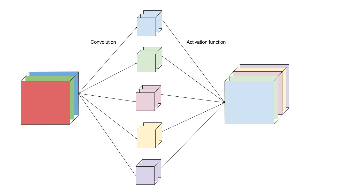
Intuitively, we can think of each filter as a “sensor” to detect a feature from the input image. For example, an edge-detecting filter is “activated” and outputs a high pixel value.

Performing convolutions on images instead of connecting each pixel to the neural network units has two main advantages:

1. Reduces the number of parameters we need to learn. Instead of learning the weights connecting each input pixel, we only need to learn the weights of the filter (which usually is a lot smaller than the input image).

2. Preserves locality. We don’t have to flatten the image matrix into a vector, thus the relative positions of the image pixels are preserved. Take a cat image for example. The information that makes up a cat includes the relative positions of its eyes, nose, and fluffy ears. We lose that insight if we represent the image as one long string of numbers.

Intuitively, we can imagine each convolution of a filter on an image as gathering and processing the information on one part of the image and sum them up into a single, meaningful value.

Padding

What do we do if the filter does not perfectly “fit” the input image? Well, we have two options:

1. Pad the picture with zeros (zero-padding) such that it fits, or

2. Drop the part of the image where the filter didn’t fit. This is called valid-padding, keeping only the valid part of the image.

Another problem with convolution is that the dimension of the image is reduced. If we pass the input through many convolution layers without padding, the image size shrinks and eventually becomes too small to be useful.

The solution to this is to apply zero-padding to the image such that the output has the same width and height as the input. This is formally called same-padding.

Strides

The next parameter we can choose during convolution is known as stride. Stride means the number of pixels our filter will move each time. Most of the examples that you have seen before have a stride of one. The picture below shows how convolution would work with a stride of 2.

It might bother you now why we would like to change the stride. This is because it could help reduce the image. With a stride of 1, our output from above would result in a 5x5 image. However, with a stride of 2, we would get a 3x3 image instead. For some images where close pixel values are quite similar, we do not need to sample every pixel since we could obtain the same information with a smaller image.

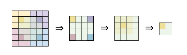
Pooling Layer

After the convolutional layer, it is a common practice to pass these values into the next layer which is known as the pooling layer. What pooling does is applying a special kind of filter to your output where the two most common form is max and average pooling. With max pooling, this is like applying a max filter on the image. This is also the same for the average pooling.

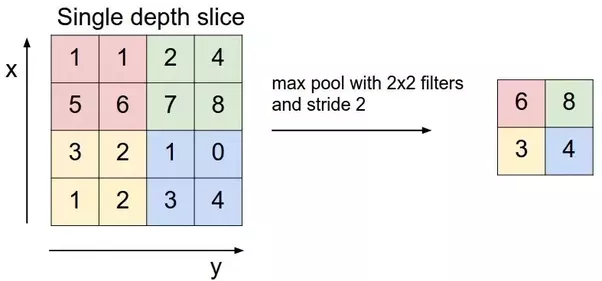
The reason why we use the pooling layer is again to reduce the size of the data. With max or average pooling, we are able to still preserve the image information with a smaller image. People generally prefer max pooling over average pooling when dealing with computer vision because it produces better results, but we still do not know why.

Fully Connected Layer

After the pooling layer, we flattened our data into a vector and feed it into a fully connected layer like in a normal neural network. We have this layer in order to add non-linearity to our data. If to give an example of a human face, the convolutional layer might be able to identify features like faces, nose, ears, and etc. However, they do not know the position or where these features should be. With the fully connected layers, we combined these features together to create a more complex model that could give the network more prediction power as to where these features should be located in order to classify it as human. Finally, we have an activation function such as a softmax or sigmoid that outputs our result. This might not be obvious to you yet but later we will be able to remove these fully connected layers and have a fully convolutional layer instead. However, let’s leave that for later.

CNN Recap

We know that that is a lot of information to take so let us recap from the beginning how CNN works again.

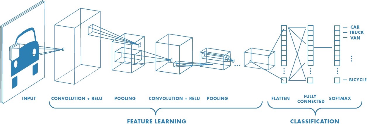
1. Feed our input image into the convolutional layer.
2. Convolutional layer. Choose parameters for convolution including stride, padding, and filter size. Perform convolution on the image. Perform a ReLU activation on the whole matrix. Perform pooling on the output to reduce the size. Add as many convolutional layers until satisfied.
3. Flatten the output and feed into a fully-connected layer.
4. Output the class using an activation function such as softmax or sigmoid function

Even if after you read through our article and still find yourself confused about CNN or neural network in general, that is ok. These concepts and math are quite hard to get in the first go. However, this is one of the magic of neural network. By just understanding the big picture, you will be able to produce satisfying results. In our next post, we would like to introduce to you the tools that would allow you to build your CNN without the mathematics intuition and also show some really popular models that people have built. See you next time.