It is undeniable that Convolutional Neural Networks (CNN) have made a huge progress in the field of computer vision. Most state-of-the-art models in image classification and object detection have been some form of a CNN. Convolutional Neural Networks work by convolving pixels of image data, down-sampling, and applying non-linearity after each successive layer. The result is called a “feature map” or a learned abstraction of an image. What does it learn? It is hard to quantify concretely what a deep learning model learns. However, it is generally known via visualizing weights and layer activations that feature maps earlier in the network learns the general concepts of an image — for example, edges, colors, and shapes — and that feature maps later in the network learns the specifics (e.g. pixel-level features) of an image. The last feature map of an image may be fed into a classifier (e.g. SVM, Feed Forward Neural Network) to output a probability of an image being in a class.

Transfer learning is a popular technique in deep learning where one may use a pre-trained model learned in one task, and fine-tune the weights to fit on a new dataset. This technique works very well in practice because it allows the network to use the features it previously learned, mix and match them in new combinations, and use it to classify a new set of images. In fact, it is generally accepted that one should never train a CNN from scratch anymore. Thanks to the ImageNet dataset, people have made lots of pre-trained models where these models are trained over millions of images to solve the specific task of classification of a thousand classes of images. The result is a model that is rich in pre-trained features and has lots of understanding of images in general (e.g. features of cars, animals, trees, tools, etc.). In practice, transfer learning works much better than training a model from random initialisation: the model converges much faster, and in many cases more accurate.

For the remainder of this post, I will be stepping through a simple example of dogs vs. cat image classification. The details of this dataset and its goals can be found here https://www.kaggle.com/c/dogs-vs-cats. Basically, I have 25,000 images labeled as dogs or cats. I want to train a CNN so that it is able to classify new images it has never seen as dogs or cats. First, let’s import the necessary tools and load the data:

import os
import random
import numpy as np
from scipy.ndimage import imread
from scipy.misc import imresize
from keras.models import Model
from keras.callbacks import ModelCheckpoint
from keras.layers import Input, Conv2D, MaxPooling2D, UpSampling2D, GlobalAveragePooling2D, Dense
from keras.applications.inception_v3 import InceptionV3
from keras.utils import to_categorical
filenames = []
labels = []
for filename in os.listdir("./images"):
    filenames.append(os.path.join("./images/", filename))
    labels.append(filename.split(".")[0])
zipped = list(zip(filenames, labels))
random.shuffle(zipped)
filenames, labels = zip(*zipped)
X_train = filenames[0:int(len(filenames)*0.8)]
y_train = labels[0:int(len(filenames)*0.8)]
X_val = filenames[int(len(filenames)*0.8):]
y_val = labels[int(len(filenames)*0.8):]

The images are given in a single directory (here I named it “images”). The label is given in the name. For example, an image of a cat might be cat.XXXX.jpg where XXXX is some number. Essentially, I have made a shuffled list of filenames and the label either as “cats” or “dogs”. Then, the data is split into 80% training and 20% validation.

Next, we create a custom image data generator. Keras has a class ImageDataGenerator, but we would need to have our images structured in directories in a very specific way. With this custom image data generator, it will generate a batch of images of size (224, 224, 3) into a numpy array of shape (batch_size, 224, 224, 3).

def image_generator(data_X, data_y, batch_size=64):
    X_arr = []
    y_arr = []
    while True:
        for i in range(len(data_X)):
            x = imread(data_X[i], mode="RGB")
            x_reshaped = imresize(x, (224, 224, 3))
            x_reshaped = x_reshaped / 255.
            # cat = 0, dog = 1
            y = int(data_y[i] == "dog")
            X_arr.append(x_reshaped)
            y_arr.append(y)
            if len(X_arr) == batch_size:
                X_out = np.array(X_arr)
                y_out = np.array(y_arr)
                X_arr = []
                y_arr = []
                yield (X_out, to_categorical(y_out))
bs = 64
train_data_generator = image_generator(X_train, y_train, batch_size=bs)
val_data_generator = image_generator(X_val, y_val, batch_size=bs)

Random Initialisation

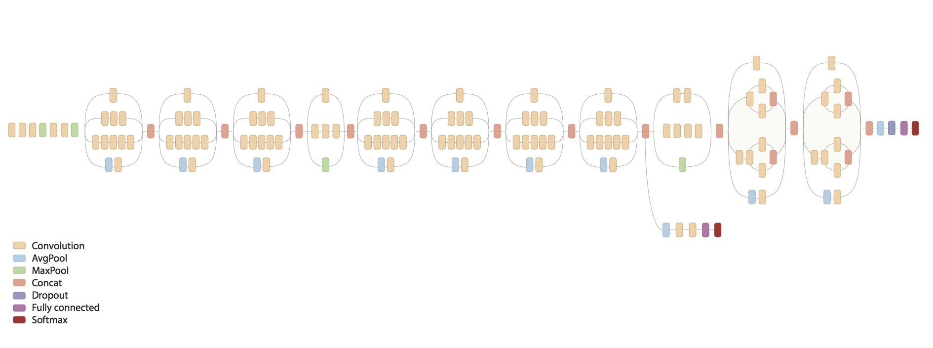
Now we can define our model. Here we will be using InceptionV3, a very successful architecture of CNN. Here we will set weights=None to demonstrate the case when we initialize the weights randomly. The output of the InceptionV3 is shaped (None, 5, 5, 2048). The output is fed into a GlobalAveragePooling2D layer to average the (5, 5, 2048) features into 2048 features, averaging the (5, 5) numbers. Essentially, you have 2048 numbers that summarizes the (224, 224, 3) image you input into the network. Next, we feed this into a Dense layer with 1024 hidden nodes before it is fed into a prediction layer with 2 nodes using the softmax activation function.

inception_v3 = InceptionV3(weights=None,
                           include_top=False, 
                           input_shape=(224,224,3))
x = inception_v3.output
x = GlobalAveragePooling2D()(x)
x = Dense(1024, activation='relu')(x)
predictions = Dense(2, activation='softmax')(x)
model = Model(inception_v3.input, predictions)

Transfer Learning

For the case of transfer learning, we can simply change weights=None to weights=”imagenet” (or simply remove it, default is imagenet). Further, I’m going to choose to freeze all the weights in InceptionV3 learned from ImageNet, and train only the Dense layer. It is possible to fine-tune the whole network and whether we do it will depend on the nature of our dataset. If the dataset is similar to ImageNet (e.g. cars, animals, trees, tools), then it may be unnecessary to fine-tune the whole network. You can read more about the best practices from here: http://cs231n.github.io/transfer-learning/.

inception_v3 = InceptionV3(weights='imagenet',
                           include_top=False, 
                           input_shape=(224,224,3))
x = inception_v3.output
x = GlobalAveragePooling2D()(x)
x = Dense(1024, activation='relu')(x)
predictions = Dense(2, activation='softmax')(x)
model = Model(inception_v3.input, predictions)
for layer in inception_v3.layers:
    layer.trainable = False
model.compile(optimizer='adam', 
              loss='categorical_crossentropy',
              metrics=['acc'])

Results

Let us now compare the accuracies and the time it takes to train these models. Below is the training run for the case of random initialization:

Epoch 00091: val_acc did not improve
Epoch 92/100
312/312 [==============================] - 145s 464ms/step - loss: 2.3751e-06 - acc: 1.0000 - val_loss: 0.2401 - val_acc: 0.9655
Epoch 00092: val_acc improved from 0.96534 to 0.96554, saving model to classifier.h5
Epoch 93/100
312/312 [==============================] - 145s 464ms/step - loss: 1.8455e-06 - acc: 1.0000 - val_loss: 0.2416 - val_acc: 0.9655
**Epoch 00093: val_acc did not improve
Epoch 94/100
312/312 [==============================] - 145s 464ms/step - loss: 1.5706e-06 - acc: 1.0000 - val_loss: 0.2452 - val_acc: 0.9657
Epoch 00094: val_acc improved from 0.96554 to 0.96575, saving model to classifier.h5**
Epoch 95/100
312/312 [==============================] - 145s 464ms/step - loss: 1.2430e-06 - acc: 1.0000 - val_loss: 0.2483 - val_acc: 0.9657
Epoch 00095: val_acc did not improve
Epoch 96/100
312/312 [==============================] - 145s 465ms/step - loss: 1.0860e-06 - acc: 1.0000 - val_loss: 0.2500 - val_acc: 0.9657
Epoch 00096: val_acc did not improve
Epoch 97/100
312/312 [==============================] - 145s 464ms/step - loss: 8.6695e-07 - acc: 1.0000 - val_loss: 0.2527 - val_acc: 0.9655
Epoch 00097: val_acc did not improve
Epoch 98/100
312/312 [==============================] - 145s 464ms/step - loss: 7.8315e-07 - acc: 1.0000 - val_loss: 0.2547 - val_acc: 0.9655
Epoch 00098: val_acc did not improve
Epoch 99/100
312/312 [==============================] - 145s 464ms/step - loss: 6.2808e-07 - acc: 1.0000 - val_loss: 0.2568 - val_acc: 0.9655
Epoch 00099: val_acc did not improve
Epoch 100/100
312/312 [==============================] - 145s 464ms/step - loss: 5.6699e-07 - acc: 1.0000 - val_loss: 0.2568 - val_acc: 0.9655

Validation accuracy reached its highest at epoch 94 at 96.56%. Total training time is roughly 4 hours with a single NVIDIA GTX 1080 TI. The accuracy could probably go higher as it seem to still be increasing slowly. Further, we could tune our training by adding dropout regularization to reduce overfitting, add more Dense layer(s) before the prediction layer, tune the number of hidden nodes of each Dense layer, or change the optimizing method (e.g. rmsprop, SGD, change batch size, change learning rates, etc). I encourage you to experiment with these ideas!

Now let’s look at the result for the case of transfer learning.

Epoch 1/100
312/312 [==============================] - 92s 296ms/step - loss: 0.1918 - acc: 0.9198 - val_loss: 0.0982 - val_acc: 0.9728
Epoch 00001: val_acc improved from -inf to 0.97276, saving model to classifier.h5
Epoch 2/100
312/312 [==============================] - 91s 291ms/step - loss: 0.1266 - acc: 0.9479 - val_loss: 0.0896 - val_acc: 0.9756
Epoch 00002: val_acc improved from 0.97276 to 0.97556, saving model to classifier.h5
Epoch 3/100
312/312 [==============================] - 91s 292ms/step - loss: 0.1132 - acc: 0.9531 - val_loss: 0.0733 - val_acc: 0.9816
Epoch 00003: val_acc improved from 0.97556 to 0.98157, saving model to classifier.h5
Epoch 4/100
312/312 [==============================] - 91s 292ms/step - loss: 0.0928 - acc: 0.9639 - val_loss: 0.0679 - val_acc: 0.9832
Epoch 00004: val_acc improved from 0.98157 to 0.98317, saving model to classifier.h5
Epoch 5/100
312/312 [==============================] - 92s 293ms/step - loss: 0.0786 - acc: 0.9681 - val_loss: 0.0952 - val_acc: 0.9798
Epoch 00005: val_acc did not improve
Epoch 6/100
312/312 [==============================] - 91s 292ms/step - loss: 0.0625 - acc: 0.9769 - val_loss: 0.1265 - val_acc: 0.9774
Epoch 00006: val_acc did not improve
Epoch 7/100
312/312 [==============================] - 91s 293ms/step - loss: 0.0560 - acc: 0.9787 - val_loss: 0.0980 - val_acc: 0.9830
Epoch 00007: val_acc did not improve
Epoch 8/100
312/312 [==============================] - 91s 293ms/step - loss: 0.0463 - acc: 0.9830 - val_loss: 0.0754 - val_acc: 0.9868
Epoch 00008: val_acc improved from 0.98317 to 0.98678, saving model to classifier.h5
Epoch 9/100
312/312 [==============================] - 92s 294ms/step - loss: 0.0465 - acc: 0.9818 - val_loss: 0.0738 - val_acc: 0.9868
Epoch 00009: val_acc did not improve
Epoch 10/100
312/312 [==============================] - 91s 292ms/step - loss: 0.0528 - acc: 0.9791 - val_loss: 0.0731 - val_acc: 0.9870
Epoch 00010: val_acc improved from 0.98678 to 0.98698, saving model to classifier.h5
Epoch 11/100
312/312 [==============================] - 91s 293ms/step - loss: 0.0580 - acc: 0.9743 - val_loss: 0.0830 - val_acc: 0.9866
Epoch 00011: val_acc did not improve
Epoch 12/100
312/312 [==============================] - 91s 293ms/step - loss: 0.0588 - acc: 0.9769 - val_loss: 0.1921 - val_acc: 0.9718
Epoch 00012: val_acc did not improve
Epoch 13/100
312/312 [==============================] - 91s 292ms/step - loss: 0.0552 - acc: 0.9782 - val_loss: 0.1874 - val_acc: 0.9762
Epoch 00013: val_acc did not improve
Epoch 14/100
312/312 [==============================] - 92s 294ms/step - loss: 0.0416 - acc: 0.9835 - val_loss: 0.1687 - val_acc: 0.9778
Epoch 00014: val_acc did not improve
Epoch 15/100
312/312 [==============================] - 91s 292ms/step - loss: 0.0320 - acc: 0.9875 - val_loss: 0.1464 - val_acc: 0.9804
Epoch 00015: val_acc did not improve
Epoch 16/100
312/312 [==============================] - 91s 293ms/step - loss: 0.0241 - acc: 0.9916 - val_loss: 0.1786 - val_acc: 0.9766
Epoch 00016: val_acc did not improve
Epoch 17/100
312/312 [==============================] - 91s 293ms/step - loss: 0.0186 - acc: 0.9941 - val_loss: 0.1482 - val_acc: 0.9842
Epoch 00017: val_acc did not improve
Epoch 18/100
312/312 [==============================] - 91s 293ms/step - loss: 0.0157 - acc: 0.9949 - val_loss: 0.1401 - val_acc: 0.9834
Epoch 00018: val_acc did not improve
Epoch 19/100
312/312 [==============================] - 91s 291ms/step - loss: 0.0186 - acc: 0.9937 - val_loss: 0.2895 - val_acc: 0.9665
Epoch 00019: val_acc did not improve
Epoch 20/100
312/312 [==============================] - 91s 293ms/step - loss: 0.0194 - acc: 0.9929 - val_loss: 0.1065 - val_acc: 0.9868
Epoch 00020: val_acc did not improve
Epoch 21/100
312/312 [==============================] - 91s 292ms/step - loss: 0.0172 - acc: 0.9938 - val_loss: 0.1616 - val_acc: 0.9820
Epoch 00021: val_acc did not improve
Epoch 22/100
312/312 [==============================] - 91s 293ms/step - loss: 0.0188 - acc: 0.9932 - val_loss: 0.1071 - val_acc: 0.9868
Epoch 00022: val_acc did not improve
**Epoch 23/100
312/312 [==============================] - 91s 292ms/step - loss: 0.0199 - acc: 0.9931 - val_loss: 0.0898 - val_acc: 0.9884
Epoch 00023: val_acc improved from 0.98698 to 0.98838, saving model to classifier.h5**

Notice that the validation accuracy beats that of random initialization after the first epoch. In 91 seconds, we were able to beat a 4-hour long training…! After 23 epochs (34 minutes), we tested the model on a different Kaggle competition on cats vs. dogs (link: https://www.kaggle.com/c/skoltech-cats-vs-dogs/submissions?sortBy=date&group=all&page=1), and the model gets 99.25% test accuracy (#2 on the public leaderboard). This suggests that our model is accurate and generalizes well to other datasets.

As I have shown, transfer learning not only gives better prediction results, but it also trains faster. Transfer learning is probably a more realistic way in which humans learn; we don’t relearn everything from scratch every time we are given a new task, but we build on top of the knowledge we already have. Aside from computer vision, transfer learning have been very successful in Natural Language Processing as well. For example, a form of pre-training in NLP is when words are made vectors by a process called Word2Vec. With transfer learning, we are building an intelligent AI by building on top of existing knowledge, datasets after datasets, accumulating knowledge over time. Transfer learning has brought us so far, and looking forward, I believe that it is where AI is headed.